Data Mining is one of the many buzzwords floating about in the data science ether, a noun high on enthusiasm, but typically low on specifics. It is often described as a cross between statistics, analytics, and machine learning (yet another buzzword). Data mining is not, as is often believed, a process that extracts data. It is more accurate to say that data mining is a process of extracting unobserved patterns from data. Such patterns and information can represent real value in unlikely circumstances.

Those who work in economics and the law may find themselves confused by, and suspicious of, the latest fads in computer science and analytics. Indeed, concepts in econometrics and statistics are already difficult to convey to judges, juries, and the general public. Expecting a jury composed entirely of mathematics professors is fanciful, so the average economist and lawyer must find a way to convincingly say that X output from Y method is reliable, and presents an accurate account of the facts. In that instance, why make a courtroom analysis even more remote with “data mining” or “machine learning”? Why risk bamboozling a jury, especially with concepts that even the expert witness struggles to understand? The answer is that data mining and machine learning open up new possibilities for economists in the courtroom, if used for the right reasons and articulated in the right manner.

Consider the following case study:

A class action lawsuit is filed against a major Fortune 500 company, alleging gender discrimination. In the complaint, the plaintiffs allege that female executives are, on average, paid less than men. One of the allegations is that starting salaries for women are lower than men, and this bias against women persists as they continue working and advancing at this company. After constructing several different statistical models, the plaintiff’s expert witness economist confirms that the starting salaries for women are, on average, several percentage points lower than men. This pay gap is statistically significant, the findings are robust, and the regressions control for a variety of different employment factors, such as the employee’s department, age, education, and salary grade.

However, the defense now raises an objection in the following vein: “Of course men and women at our firm have different starting salaries. The men we hire tend to have more relevant prior job experience than women.” An employee with more relevant experience would (one would suspect) be paid more than an employee with less relevant prior experience. In that case, the perceived pay gap would not be discriminatory, but a result of an as-of-yet unaccounted variable. So, how can the expert economist quantify relevant prior job experience?

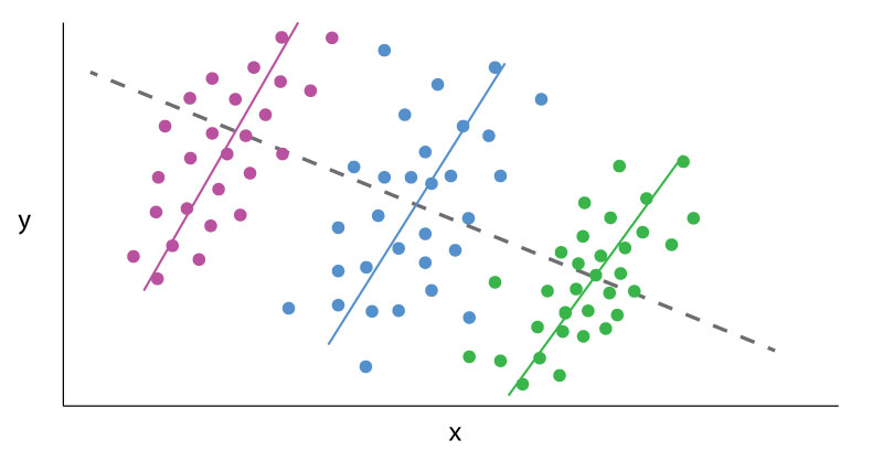
For larger firms, one source could be the employees’ job applications. In this case, each job application was filed electronically and can be read into a data analytics programs. These job applications list the last dozen job titles the employee held, prior to their position at this company. Now the expert economist lets out a small groan. In all, there are tens of thousands of unique job titles. It would be difficult (or if not difficult, silly) to add every single prior job title as a control in the model. So, it would make sense to organize these prior job titles into defined categories. But how?

This is one instance where new techniques in data science come into play.

The 2020 coronavirus outbreak has sparked severe shocks to the United States labor market. Social distancing policies, designed to slow the spread of the disease, are leading to large layoffs in specific industries, like bars and restaurants. Many more employees in other sectors face the prospect of unemployment or temporary furloughs. Despite this economic strain, employers, particularly those in Medical and Supply Chain services, are expanding to meet new demand. These sectors continue to post job opportunities long after policymakers mandated the closure of non-essential services or issued “shelter-in-place” orders.

Evidence from Texas over the past half-month reveals both predictable and unexpected trends in new job opportunities. It may come as a surprise that, even in this “lockdown economy,” there is still help wanted.

Beginning on March 18th, Texas began implementing statewide social distancing policies, though some areas began issuing such orders days earlier. Cities and counties across the state gradually adopted “shelter-in-place” orders in March.  By March 31st, a statewide order asked residents to stay home, except if they participated in “essential services and activities.”

But within the past two weeks, Texas employers posted over 66,000 new job openings.

Daily job postings are one indicator of up-to-date labor market demand, available from a variety of sources (most notably online).  The Texas Workforce Commission (“TWC”) is the state agency responsible for managing and providing workforce development services to employers and potential employees in Texas.  One service the TWC provides is access to databases of up-to-date job postings for different occupations and employers within the state. These job postings can come from the TWC itself, or from third party sites like Monster or Indeed. This information is extraordinarily valuable to data scientists.

The top 10 in demand occupations cover a variety of occupations, but are heavily concentrated in the healthcare, supply chain, and IT sectors.

Given the stresses to the healthcare system, its little surprise that hospitals are looking for more front-line staff. Registered Nurses were the highest in demand occupation, with over 3,000 new job listings since March 23rd.

 

Retail supply chains are also expanding employment.  Sales Representatives for Wholesalers and Manufacturers, with over 2,300 new listings, was the second highest in demand occupation. Other logistical occupations saw large numbers of new openings, particularly for Truck Drivers, with over 1,200 new job postings since March 23rd.

Anecdotally, supermarkets and retail chains have been hiring more employees to meet increased demand for groceries and other supplies. Evidence from jobs posted since March 23rd would support this finding, with large increases in new listings for Customer Service Representatives (over 1,700), Supervisors of Retail Sales Workers (over 1,600), and Retail Salespersons (also over 1,600).

Finally, with the increase in service sector employees working from home, it should not be surprise that IT workers are also in high demand. Application Developers (over 2,100 new listings) and employees for general Computer Occupations (with 1,800 new listings) have both seen large increases in openings since March 23rd.

EmployStats will be closely monitoring daily job postings as the coronavirus outbreak continues.

Data Analytics can sometimes be a frustrating game of smoke and mirrors, where outputs change based on the tiniest alterations in perspective. The classic example is Simpson’s paradox.

Simpson’s paradox is a common statistical phenomenon which occurs whenever high-level and subdivided data produce different findings. The data itself may be error free, but how one looks at it may lead to contradictory conclusions. A dataset results in a Simpson’s paradox when a “higher level” data cut reveals one finding, which is reversed at a “lower level” data cut. Famous examples include acceptance rates by gender to a college, which vary by academic department, or mortality rates for certain medical procedures, which vary based on the severity of the medical case. The presence of such a paradox does not mean one conclusion is necessarily wrong; rather, the presence of a paradox in the data warrants further investigation.

“Lurking variables” (or “confounding variables”) are one key to understanding Simpson’s paradox. Lurking variables are those which significantly affect variables of interest, like the outputs in a data set, but which are not controlled for in an analysis. These lurking variables often bias analytical outputs and exaggerate correlations. However, improperly “stratifying data” is also key to Simpson’s paradox. Aggressively sub-dividing data into statistically insignificant groupings or controlling for unrelated variables can generate inconclusive findings. Both forces operate in opposing directions. The solution to the paradox is to find the data cut which is most relevant to answering the given question, after controlling for significant variables.

EmployStats recently worked on an arbitration case out of Massachusetts, where the Plaintiffs alleged that a new evaluation system negatively impacted older and minority teachers more than their peers in a major public school district. One report provided by the Defense examined individual evaluators in individual years, arguing that evaluators were responsible for determining the outcome of teacher evaluations. This report determined, based on that data cut, the new evaluation system showed no statistical signs of bias. By contrast, the EmployStats team systematically analyzed all evaluations, controlling for different factors such as teacher experience, the type of school, and student demographics. The team found that the evaluations, at an overall level and after controlling for a variety of variables, demonstrated a statistically significant pattern of biases against older and minority teachers.

The EmployStats team then examined the Defense’s report. The team found that if all the evalulator’s results were jointly tested, the results showed strong, statistically significant biases against older and minority teachers, which matched the Plaintiff’s assertions. If the evaluators really were a lurking variable, then specific evaluators should have driven a significant number of results. Instead, the data supported the hypothesis that the evaluation system itself was the cause of signs of bias.

To see how EmployStats can assist you with similar statistics cases, please visit www.EmployStats.com or give us a call at 512-476-3711.  Follow our blog and find us on social media: @employstatsnews

Civil fraud cases hinge on litigants proving where specific fraudulent activity occurred. Tax returns, sales records, expense reports, or any other large financial data set can be manipulated. In many instances of fraud, the accused party diverts funds or creates transactions, intending to make their fraud appear as ordinary or random entries. More clever fraudsters ensure no values are duplicated or input highly specific dollar and cent amounts. Such ‘random’ numbers, to them, may appear normal, but few understand or replicate the natural distribution of numbers known as Benford’s Law.

A staple of forensic accounting, Benford’s Law is a useful tool for litigants in establishing patterns of fraudulent activity.

Benford’s Law states that, for any data set of numbers, the number 1 will be the leading numeral about 30% of the time, the number 2 will be the leading numeral about 18% of the time, and each subsequent number (3-9) will be a leading number with decreasing frequency.  This decreasing frequency of numbers, from 1 though 9, can be represented by a curve that looks like this:

For example, according to Benford’s Law, one would expect that more street addresses start with a 1 than a 8 or 3; such hypothesis can be tested and proven. The same pattern holds for any number of phenomenon: country populations, telephone numbers, passengers on a plane, or the volumes of trades. This predicted distribution permeates many aspects of numbers and big data sets. But Benford’s Law is not absolute: it does require larger data sets, and that all the leading digits (1-9) must have a theoretically equal chance of being the leading digit. Benford’s Law, for example, would not apply to a data set where only 4s or 9s are the leading number. Financial data sets do comport with a Benford distribution.

In accounting and financial auditing, Benford’s Law is used to test a data set’s authenticity. False transaction data is typically tampered by changing values or adding additional fake data. The test, therefore, is an early indicator if a data set has been altered or artificially created. Computer generated random numbers will tend to show an equal distribution of leading digits. Even manually created false entries will tend to have some sort of underlying pattern. A person may, for example, input more fake leading digits based on numbers closer to their typing fingers (5 and 6).

An examiner would compare the distribution of leading digits in the data set, and the Benford distrubtion. Then, the examiner would statistically test if the proportion of leading numbers in the data set matches a Benford distribution. The resulting “Z-scores” give a measure of how distorted these distributions are, with higher “Z-scores” implying a more distorted data set, which implies artificially created data.

If a data set violates Benford’s Law, that alone does not prove such transactions numbers fraudulent. But, a violation does give auditors, economists, and fact finders an additional reason to scrutinize individual transactions.

This series on data analytics in litigation emphasized how best practices help secure reliable, valid, and defensible results based off of “Big Data.” Whether it is inter-corporate litigation, class actions, or whistleblower cases, electronic data is a source of key insights. Courts hold wide discretion in admitting statistical evidence, which is why opposing expert witnesses scrutinize or defend results so rigorously. There is generally accepted knowledge on the techniques, models, and coding languages for generating analytical results from “Big Data.” However, the underlying assumptions of a data analysis are biased. These assumptions are largest potential source of error, leading parties to confuse, generalize, or even misrepresent their results. Litigants need to be aware of and challenge such underlying assumptions, especially in their own data-driven evidence.

 

When it comes to big data cases, the parties and their expert witnesses should be readily prepared with continuous probing questions. Where (and on what program) are the data stored, how they are interconnected, and how “clean” they are, directly impact the final analysis. These stages can be overlooked, leading parties to miss key variables or spend additional time cleaning up fragmented data sets. When the data are available, litigants should not miss on opportunities due to lack of preparation or foresight. When data do not exist or they do not support a given assertion, a party should readily examine its next best alternative.

 

When the proper analysis is compiled and presented, the litigating parties must remind the court of the big picture: how the analysis directly relates to the case. Do the results prove a consistent pattern of “deviation” from a given norm? In other instances, an analysis referencing monetary values can serve as a party’s anchor for calculating damages.

 

In Big Data cases, the data should be used to reveal facts, rather than be molded to fit assertions.

For data-based evidence, the analysis is the heart of the content: the output of the data compiled for a case. In most instances, the analytics do not need to be complex. Indeed, powerful results can be derived by simply calculating summary statistics (mean, median, standard deviation). More complicated techniques, like regressions, time-series models, and pattern analyses, do require a background in statistics and coding languages. But even the most robust results are ineffective if an opposing witness successfully argues they are immaterial to the case. Whether simple or complex, litigants and expert witnesses should ensure an analysis is both relevant and robust against criticism.

 

What type of result would provide evidence of a party’s assertion? The admissibility and validity of statistical evidence varies by jurisdiction. In general, data-based evidence should be as straightforward as possible; more complex models should only be used when necessary. Superfluous analytics are distractions, leading to expert witnesses “boiling the ocean” in search of additional evidence. Additionally, courts still approach statistical techniques with some skepticism, despite their acceptance in other fields.

 

If more complex techniques are necessary, like regressions, litigants must be confident in their methods. For example, what kind of regression will be used? Which variables are “relevant” as inputs? What is the output, and how does it relate to a party’s assertion of fact? Parties need to link outputs, big or small, to a “therefore” moment: “the analysis gave us a result, therefore it is proof of our assertion in the following ways.” Importantly, this refocuses the judge or jury’s attention to the relevance of the output, rather than its complex derivation.

 

Does the analysis match the scope of the complaint or a fact in dispute? Is the certified class all employees, or just a subset of in a company? Is the location a state, or a county within a state? If the defendant is accused of committing fraud, for how many years? Generalizing from a smaller or tangential analysis is inherently risky, and an easy target for opposing witnesses. If given a choice, avoid conjecture. Do not assume that an analysis in one area, for one class, or for one time automatically applies to another.

 

A key component of analytical and statistical work is replicability. In fields such as finance, insurance, or large scale employment cases, the analysis of both parties should be replicable. Outside parties should be able to analyze the same data and obtain the same results. In addition, replicability can expose error, slights of hand, or outright manipulation.

 

Data-based evidence requires focus, clarity, and appropriate analytical techniques, otherwise an output is just another number.

After acquiring and merging data, litigants will want to rush to an analysis. But raw datasets, no matter how perfectly constructed, are inevitably riddled with errors. Such errors can potentially bias or invalidate results. Data cleaning, the process which ensures a slice of data is correct, consistent, and usable, is a vital step for any data-based evidence.

 

There is a often quoted rule in data science which says 80% of one’s time is spent cleaning and manipulating data, while only 20% is spent actually analyzing it. Spelling mistakes, outliers, duplicates, extra spaces, missing values, the list of potential complications is near infinite. Corrections should be recorded at every stage, ideally in scripts of the program being used (ex. R, SAS, SQL, STATA); data cleaning scripts leave behind a structured, defensible record. Different types of data will require different types of cleaning, but a structured approach will produce error free analytical results.

 

One should start with simple observations. Look at batches of random rows, what values are stored for a given variable, and are these values consistent? Some rows may format phone numbers differently, inconsistently capitalize, or round values. How many values are null, and are there patterns in null entries? Calculate summary statistics for variables, are there obvious mistakes (ex. negative time values)? After an assessment, cleaning can begin.

 

Fixing structural errors is straightforward: input values with particular spellings, capitalization, split values (ex. data containing ‘N/A’ and ‘Not Available’), or formatting issues (ex. numbers stored as strings rather than integers) can be systematically reformatted. Duplicate observations, common when datasets are merged, can be easily removed.

 

However, data cleaning is not entirely objective. Reasonable assumptions must be made when handling irrelevant observations, outliers, and missing values. If class X or transaction type Y is excluded from litigation, its reasonable to remove their observations. However, one cannot automatically assume Z, a similar class, can be removed as well. Outliers function the same way. What legal reasoning do I have to remove this value from my dataset? Suspicious measurements are a good excuse; but, just because a value is too big or too small, that alone does not make it reasonable to remove.

 

Missing data is a difficult problem: how many missing or null values are acceptable for this analysis to still produce robust results? Should you ignore missing values, or should you generate values based off of similar data points? There is no easy answer.  Both approaches assume missing observations are similar to the rest of the dataset. But the fact that the observations are missing data is informative in of itself. A more cautious stance, the one with the least assumptions, will inevitably be easier to defend in court.

 

Skipping data cleaning, and assuming perfect data, casts doubt on any final product. Data-based evidence follows the maxim “garbage in, garbage out.”

Data analytics is only beginning to tap into the unstructured data which forms the bulk of everyday life. Text messages, emails, maps, audio files, PDF files, pictures, blog posts, these sources represent ‘unstructured data,’ as opposed to the structured data sources mentioned thus far. Up to 80% of all enterprise data is unstructured. So, how can a client’s text messages or recorded phone calls be analyzed like a SQL table? Unstructured data is not easily stored into pre-defined models or schema; some CRM tools (e.x. Salesforce) do store text-based fields. But typically, documents do not lend themselves to traditional queries from a database. This does not mean ‘structured’ and ‘unstructured’ data are in conflict with each other.

 

Document based evidence is of course, an integral part of the legal system. Lawyers and law offices now have access to comprehensive e-discovery programs, which sift through millions of documents based on keywords and terms. Selecting relevant information to prove a case is nothing new. The intersection with Data Analytics arises when hundreds of thousands or millions of text based data are analyzed as a whole, to prove an assertion in court.

 

Turning unstructured text into analyzable, structured data is made possible by increasingly sophisticated methods. Some machine learning algorithms, for example, analyze pictures and pick up on repeating patterns. Text mining programs scrape PDFs, websites, and social media for content, and then download the text into preassigned columns and variables. Analyses can be run, for example, on the positivity or negativity of a sentence, the frequency of certain words, or the correlation of certain phrases to one another. Natural language processing (NLP) includes speech recognition, which itself has seen significant progress in the past two decades. Analytics on unstructured data is now more useful in producing relevant evidence.

 

As important as the unstructured data is its corresponding Metadata: data that describes data. A text message or email contains additional information about itself: for example the author, the recipient, the time, and the length of the message. These bits of information can be stored in a structured data set, without any reference to the original content, and then analyzed. For example, a company has metadata on electronic documents at specific points in a transaction’s life-cycle; running a pattern analysis on this metadata could identify whether or not certain documents were made, altered, or destroyed after an event.

 

In instances of high profile fraud, such as the London Inter-bank Offered Rate (LIBOR) manipulation scandal, prolific emails and text messages between traders added a new dimension to the regulator’s cases against major banks. Overwhelming and repeated textual evidence, which can be produced through analyses on unstructured data, is yet another tool for litigating parties to prove a pattern of misconduct.

Due to the massive computational requirements of analyzing big data, trying to find the best approach to big data projects can be a daunting task for most individuals.  At EmployStats, our team of experts utilize top of the line data systems and software to seamlessly analyze big data and provide our clients with high quality analysis as efficiently as possible.

1. The general approach for big data analytics begins with fully understanding the data provided as a whole.  Not only must the variable fields in the data be identified, but one must also understand what these variables represent and determine what values are reasonable for each variable in the data set.  
2. Next, the data must be cleaned and reorganized into the clearest format, ensuring that data values are not missing and are within reasonable ranges of certainty.  As the size of the data increases, the amount of work necessary to clean the data increases.  In larger datasets there are more individual components which are typically dependent on each other, therefore it is necessary to write computer programs to evaluate the accuracy of the data.
3. Once the entire dataset has been cleaned and properly formatted, one needs to define the question that will be answered with the data.  One must look at the data and see how it relates to the question.  The questions for big data projects may be related to frequencies, probabilities, economic models, or any number of statistical properties.  Whatever it is, one must then process the data in the context of the question at hand.
4. Once the answer has been obtained, one must determine that the answer is a strong answer.  A delicate answer, or one that would significantly change if the technique of the analysis was altered, is not ideal.  The goal of big data analytics is to have a robust answer, and one must try to attack the same question in a number of different ways in order to build confidence in the answer.