statistical analysis – Economic Thinking In Action

Data Analytics and the Law: Acquiring Data

Evidence based on Data Analytics hinges on the relevance of its underlying sources. Determining what potential data sources can prove is as important as generating an analysis. The first question should be “What claims do I want to assert with data?” The type of case and nature of the complaint should inform litigants where they should start looking in discovery. For example, a dataset of billing information could determine whether or not a healthcare provider committed fraud. Structured data sources like Excel files, SQL servers, or third party databases (e.x. Oracle), are the primary source material for statistical analyses, particularly those using transactional data.

In discovery, it’s important that both parties be aware of these structured data sources. Often, these sources do not have a single designated custodian, rather they may be the purview of siloed departments or an IT group. For any particular analysis, rarely is all the necessary data all held in one place. Identifying valuable source material is more difficult as the complexity of interactions between different sources increases. To efficiently stitch together smaller databases and tables, a party should conduct detailed data mapping by identifying links between structured data sources. For example, how two tables relate to another, how a SQL table relates to an Excel file, or how a data cube relates to a cloud file. Data mapping identifies which structured data sources are directly linked to one another through their variables, and how they as a whole fit together in an analysis.

However when using data based evidence to answer a question, structured data is rarely clean and/or well organized. Variables defined in a table may be underutilized or unused. Legacy files imported into newer systems can become corrupted. The originators of macros or scripts for data pulls may no longer work for an organization and forgo detailed instructions. Sometimes the data simply do not exist: not from a party burying evidence, but by the very nature of electronically stored information (ESI).

Any defensible analysis is inherently limited by what data is available. With data analytics the maxim “evidence of absence, is not absence of evidence,” is apparent. It’s always more dangerous to exaggerate or generalize from the available data than to produce a narrow, but statistically sound result. Thus, given the data available, what questions can be asked? What questions can be answered? Finally, if there is no data, does it mean there is no problem?

Data Analytics and the Law: The Big Picture

With businesses and government now firmly reliant on electronic data for their regular operations, litigants are increasingly presenting data-driven analyses to support their assertions of fact in court. This application of Data Analytics, the ability to draw insights from large data sources, is helping courts answer a variety of questions. For example, can a party establish a pattern of wrongdoing based on past transactions? Such evidence is particularly important in litigation involving large volumes of data: business disputes, class actions, fraud, and whistleblower cases. The use cases for data based evidence increasingly cuts across industries, whether its financial services, education, healthcare, or manufacturing.

Given the increasing importance of Big Data and Data Analytics, parties with a greater understanding of data-based evidence have an advantage. Statistical analyses of data can provide judges and juries with information that otherwise would not be known. Electronic data hosted by a party is discoverable, data is impartial (in the abstract), and large data sets can be readily analyzed with increasingly sophisticated techniques. Data based evidence, effectively paired with witness testimony, strengthens a party’s assertion of the facts. Realizing this, litigants engage expert witness to provide dueling tabulations or interpretations of data at trial. As a result, US case law on data based evidence is still evolving. Judges and juries are making important decisions based the validity and correctness of complex and at times contradictory analyses.

This series will discuss best practices in applying analytical techniques to complex legal cases, while focusing on important questions which must be answered along the way. Everything, from acquiring data, to preparing an analysis, to running statistical tests, to presenting results, carries huge consequences for the applicability of data based evidence. In cases where both parties employ expert witnesses to analyze thousands if not millions of records, a party’s assertions of fact are easily undermined if their analysis is deemed less relevant or inappropriate. Outcomes may turn on the statistical significance of a result, the relevance of a prior analysis to a certain class, the importance of excluded data, or the rigor of an anomaly detection algorithm. At worst, expert testimony can be dismissed.

Many errors in data based evidence, at their heart, are faulty assumptions on what the data can prove. Lawyers and clients may overestimate the relevance of their supporting analysis, or mold data (and assumptions) to fit certain facts. Litigating parties and witnesses must constantly ensure data-driven evidence is grounded on best practices, while addressing the matter at hand. Data analytics is a powerful tool, and is only as good as the user.

CLE Speaker Dwight Steward’s Statistical Guide for Employment Law

Dwight Steward, Principal Economist at EmployStats, will be a featured speaker at the upcoming employment law CLE in San Francisco on July 12, 2017. The CLE will be taking place at the Bently Reserve in downtown San Francisco, CA, and will be discussing the recent California Equal Pay Act.

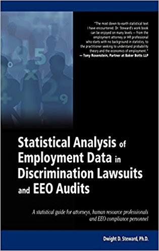
Dwight Steward, Ph.D., is the author of the book Statistical Analysis of Employment Data in Discrimination Lawsuits and EEO Audits. The statistical guide for attorneys and human resource professionals provides managers and courts with empirical evidence that goes beyond anecdotes and stories.

The textbook presents the methodologies that are used in statistical employment data analyses. The book uses a non-mathematical approach to develop the conceptual framework underlying employment data analyses, so that professionals starting with no background in statistics can easily use this book as a tool in their practice.

Visit www.CaliforniaEqualPay2017CLE.com to register to hear directly from Dwight Steward at the July 12th employment law CLE in San Francisco, CA.

Interested in purchasing Dwight Steward’s statistical guide? Find it on Amazon at www.amazon.com/Statistical-Analysis-Employment-Discrimination-Lawsuits/dp/0615340504

Using Big Data Analytics in Litigation

Due to the massive computational requirements of analyzing big data, trying to find the best approach to big data projects can be a daunting task for most individuals. At EmployStats, our team of experts utilize top of the line data systems and software to seamlessly analyze big data and provide our clients with high quality analysis as efficiently as possible.

The general approach for big data analytics begins with fully understanding the data provided as a whole. Not only must the variable fields in the data be identified, but one must also understand what these variables represent and determine what values are reasonable for each variable in the data set.
Next, the data must be cleaned and reorganized into the clearest format, ensuring that data values are not missing and are within reasonable ranges of certainty. As the size of the data increases, the amount of work necessary to clean the data increases. In larger datasets there are more individual components which are typically dependent on each other, therefore it is necessary to write computer programs to evaluate the accuracy of the data.
Once the entire dataset has been cleaned and properly formatted, one needs to define the question that will be answered with the data. One must look at the data and see how it relates to the question. The questions for big data projects may be related to frequencies, probabilities, economic models, or any number of statistical properties. Whatever it is, one must then process the data in the context of the question at hand.
Once the answer has been obtained, one must determine that the answer is a strong answer. A delicate answer, or one that would significantly change if the technique of the analysis was altered, is not ideal. The goal of big data analytics is to have a robust answer, and one must try to attack the same question in a number of different ways in order to build confidence in the answer.

Principles on statistical significance issued by American Statistical Association

The American Statistical Association released an important statement and supporting paper concerning the use and interpretation of statistical significance and p-values in statistical research.

The American Statistical Associations’ statement notes that the increased quantification of scientific research and a proliferation of large, complex data sets, often referred to as Big Data, has expanded the scope for statistics. Accordingly, the importance of appropriately chosen techniques, properly conducted analyses, and correct interpretation has also increased.

This statement by the ASA furthers, and in some ways solidifies, the ground roots “counter-statistical significance” movement that many economists and statisticians, such as Steve Zillack and Diedre McCloskey, have been working on for decades.

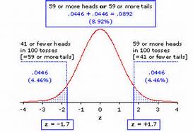
According to the ASA statement “The p-value [and the concept of statistical significance] was never intended to be a substitute for scientific reasoning,” said Ron Wasserstein, the ASA’s executive director. In research analysts use the data to calculate a p-value which shows how consistent the data is with the research hypothesis. A small p-value is typically interpreted as having a small likelihood of being consistent with the research hypothesis. In research papers, small p-values are in essence viewed as a ‘good thing’ and according to the ASA statement, are more favored by journal editors for publication.

The ASA statement argues against this approach. Instead, the ASA statement states that “Well-reasoned statistical arguments contain much more than the value of a single number and whether that number exceeds an arbitrary threshold.”

See:

Ronald L. Wasserstein & Nicole A. Lazar (2016): The ASA’s statement on p-values: context, process, and purpose, The American Statistician, DOI: 10.1080/00031305.2016.1154108

Ziliak, S.T., and McCloskey, D.N. (2008), The Cult of Statistical Significance: How the Standard Error Costs Us Jobs, Justice, and Lives, Ann Arbor: University of Michigan Press

Ziliak, S.T. (2010), “The Validus Medicus and a New Gold Standard,” The Lancet, 376, 9738, 324-325.

Perhaps one of the most useful STATA commands out there…

Working with wage and hour data and employment data, like we do on a daily basis involves the analysis of very large data sets. Big data and employment data are often one in the same. STATA has a very useful command that allows you to load in large Excel 2007/2010 spreadsheet files. It is:

set excelxlsxlargefile on

This simple command allows the user to bypass the pre-set limit on spreadsheet size.

Just remember, STATA and your computer will be unresponsive during the load. So be patient and let it all load up.

Big data question: How big of a random sample is big enough in a wage in hour case?

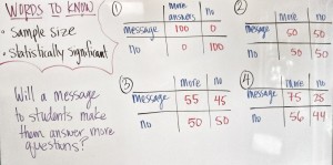
That’s a question that comes up a lot in wage and hour land employment lawsuits. Typically the question is how many employees do I need to look at to have a statistically significant sample?

In some instances it’s not feasible to collect data or get all the records for
all the employees of a particular company. Sometimes the data is kept
in such a way that it takes a lot of effort to get that information. In
other instances it is a matter of the limitations of imposed by the court.

In any event, that’s a question that comes up a number times in wage and hour lawsuits particularly ones involving class or collective actions. So what’s the answer?

Generally, the size of the sample needs to be sufficiently large so that it is representative of
the entire employee population. That number could be relatively small say 40 employees or relatively large say to 200 employees depending on the number of employees at the company and the characteristics of the employee universe that is being analyzed.

For example if there are no meaningful distinctions between the employees in the universe, that is
it is generally accepted that all the employees are pretty much all
similarly situated, then a sheer simple random sample could be
appropriate.

That is, you could simply draw names from a hat, essentially. A simple random sample typically requires the smallest number of employees.

If there are distinctions between employees that need to be accounted for, then
either a larger sample or some type of stratified sampling could be appropriate.
Even if there are distinctions between employees, if the sample is sufficiently large then distinctions between the employees in the data could take care of themselves.

For instance, assume that you have a population of 10,000 employees and they are
divided into four different groups that need to be looked at differently.

One way to do a sample in this setting is to sample over each of the different groups of employees separately. The main purpose of the individual samples is to make sure that you have the appropriate number of employees in each of the different groups. That is, to make sure that the number of employees in the different samples are sufficiently representative of the distribution of the different groups of employees in the overall population.

Another way to do this is to simply just take a large enough sample so that the distinctions take care of themselves. If the sample is sufficiently large then the distribution of the different groups of employees in the sample should on be representative of the employee population as a whole.

So in this example, if there is a sufficiently large sample it could be okay to use a simple random sample and you would get to the same point as a more advanced stratified type of approach.

The key however is to make sure that the sample is sufficiently large that of course depends on the overall population and the number of groups of employees being studied.

STATA statistical code for estimation of Millimet et al. (2002) econometric worklife model

The STATA code for estimating the Millimet et a;. (2002) econometric worklife model can be found below. The code will need to be adjusted to fit your purposes. However, the basic portions are here.

use 1992-2013, clear

drop if A_W==0
keep if A_A>=16 & A_A<86

*drop if A_MJO==0
*drop if A_MJO==14 | A_MJO==15

gen curr_wkstate = A_W>1
lab var curr_wkstate “1= active in current period”
gen prev_wkstate = prev_W>1
lab var prev_wkstate “1= active in previous period”
gen age = A_A
gen age2 = age*age
gen married = A_MA<4
gen white = A_R==1
gen male = A_SE==1

gen mang_occ = A_MJO<3
gen tech_occ = A_MJO>2 & A_MJO<7
gen serv_occ = A_MJO>6 & A_MJO<9
gen oper_occ = A_MJO>8

gen occlevel = 0
replace occlevel = 1 if mang_occ==1
replace occlevel = 2 if tech_occ==1
replace occlevel = 3 if serv_occ==1
replace occlevel = 4 if oper_occ ==1

gen lessHS = A_HGA<=38
gen HS = A_HGA==39
gen Coll = A_HGA>42
gen someColl = A_HGA>39 & A_HGA<43

gen white_age = white*age
gen white_age2 = white*age2
gen married_age = married*age

gen child_age = HH5T*age

/*
gen mang_occ_age = mang_occ*age
gen tech_occ_age = tech_occ*age
gen serv_occ_age = serv_occ*age
gen oper_occ_age = oper_occ*age
*/

merge m:1 age using mortalityrates

keep if _m==3
drop _m

gen edlevel = 1*lessHS + 2*HS + 3*someColl + 4*Coll

save anbasemodel, replace
*/ Active to Active and Active to Inactive probabilities

local g = 0
local e = 1

forvalues g = 0/1 {

forvalues e = 1/4 {

use anbasemodel, clear

xi: logit curr_wkstate age age2 white white_age white_age2 married married_age HH5T i.year_out if prev_wk==1 & male==`g’ & HS==1
*Gives you conditional probability
*summing these figures gives the average predicted probabilities

predict AAprob

keep if occlevel==`e’
*collapse (mean) AAprob mortality, by(age)

collapse (mean) AAprob mortality (rawsum) MARS [aweight=MARS], by(age)

gen AIprob = 1-AAprob

replace AAprob = AAprob*(1-mortality)
replace AIprob = AIprob*(1-mortality)

save Active_probs, replace

*Calculates Inactive first period probabiliteis

use anbasemodel, clear

xi: logit curr_wkstate age age2 white white_age white_age2 married married_age HH5T i.year_out if prev_wk==0 & male==`g’ & HS==1

predict IAprob

keep if occlevel==`e’

*collapse (mean) IAprob mortality , by(age)
collapse (mean) IAprob mortality (rawsum) MARS [aweight=MARS], by(age)

gen IIprob = 1-IAprob
save Inactive_probs, replace

*Calculates WLE for Active and Inactive

merge 1:1 age using Active_probs

drop _m

order AAprob AIprob IAprob IIprob
*Set the probablilties for end period T+1

*Note the top age changes to 80 in the later data sets
gen WLE_Active = 0
replace WLE_Active = AAprob[_n-1]*(1+AAprob) + AIprob[_n-1]*(0.5 + IAprob)
gen WLE_Inactive = 0
replace WLE_Inactive = IAprob[_n-1]*(0.5+AAprob) + IIprob[_n-1]*IAprob

gen WLE_Active_2 = 0
replace WLE_Active_2 = WLE_Active if age==85

gen WLE_Inactive_2 = 0
replace WLE_Inactive_2 = WLE_Inactive if age==85
local x = 1
local y = 80 – `x’

forvalues x = 1/63 {

replace WLE_Active_2 = AAprob*(1+WLE_Active_2[_n+1]) + AIprob*(0.5 + WLE_Inactive_2[_n+1]) if age==`y’
replace WLE_Inactive_2 = IAprob*(0.5 + WLE_Active_2[_n+1]) + IIprob*WLE_Inactive_2[_n+1] if age==`y’

local x = `x’ + 1
local y = 80 – `x’

}

keep age WLE_Active_2 WLE_Inactive_2
rename WLE_Active_2 WLE_Active_`g’_`e’
rename WLE_Inactive_2 WLE_Inactive_`g’_`e’

save WLE_`g’_`e’, replace

keep age WLE_Active_`g’_`e’
save WLE_Active_`g’_`e’, replace

use WLE_`g’_`e’, clear
keep age WLE_Inactive_`g’_`e’
save WLE_Inactive_`g’_`e’, replace

di `e’
/**End of Active to Active and Active to Inactive probabilities*/

local e = `e’ + 1
}

local g = `g’ + 1

}
local g = 0
local e = 1

forvalues g = 0/1 {

forvalues e = 1/4{

if `e’ == 1 {
use WLE_Active_`g’_`e’, clear
save WLE_Active_`g’_AllOccLevels, replace

use WLE_Inactive_`g’_`e’, clear
save WLE_Inactive_`g’_AllOccLevels, replace

}

if `e’ > 1 {

use WLE_Active_`g’_AllOccLevels, replace
merge 1:1 age using WLE_Active_`g’_`e’
drop _m
save WLE_Active_`g’_AllOccLevels, replace

use WLE_Inactive_`g’_AllOccLevels, replace
merge 1:1 age using WLE_Inactive_`g’_`e’
drop _m
save WLE_Inactive_`g’_AllOccLevels, replace

}

local e = `e’ + 1
}

if `g’ ==1 {
use WLE_Active_0_AllOccLevels, clear
merge 1:1 age using WLE_Active_1_AllOccLevels
drop _m
save WLE_Active_BothGenders_AllOccLevels, replace
use WLE_Inactive_0_AllOccLevels, clear
merge 1:1 age using WLE_Inactive_1_AllOccLevels
drop _m
save WLE_Inactive_BothGenders_AllOccLevels, replace
}

local g = `g’ + 1

}

!del anbasemodel.dta

A narrative description of the Millimet et. al (2002) econometric worklife model

The following describes the approach used by Millimet et al (2002) to estimate U.S. worker worklife expectancy. The pdf version can be found here: Millimet (2002) Methodology Description

Methodology

First, transition probabilities are obtained from a two state labor market econometric model. The two labor market states are active and inactive in the workforce. The transition probabilities are the probabilities of going from one labor market state to another, such as active in one period and inactive in the next period. There are four such transition probabilities (Active-Active, Active-Inactive, Inactive-Active, Inactive-Inactive). The transition probabilities are obtained from the conditional probabilities estimated using a standard logit frame work. The logit model states:

Where y is equal to 1 if the individual is active and y equals 0 if the individual is inactive in the workforce during the period. Logit regression models are estimated separately for active and inactive individuals. For example, for a person who is initially active, the two estimated transition probabilities (Active to Active and Active to Inactive) equations are:

The estimated transition probabilities for persons who are initially inactive are estimated in a similar manner. The transition probabilities/conditional probabilities are used to construct predicted transition probabilities for each individual in the data set.

The average of the individual predicted probabilities for each age are ultimately used to calculate the transition probabilities in the Millimet et al. (2002) econometric worklife model. The average predicted transition probabilities at each age are:

In the calculation the averages are weighted by the CPS weights. Also anine year moving average is used to smooth out the transition probabilities.

The worklife expectancy at each age can be determined recursively. Specifically, if there is an assumed terminal year (T+1) in which no one is in the workforce, then the worklife expectancy for each age prior can be determined by working backwards in the probability tree. For instance at the terminal year, the individual’s worklife in the terminal year is the worklife probability in that terminal year. For example, assume that after age 80 no individuals are active in the work force. In this example, the probability that a person who is active at age 79 will be active at age 80, is the worklife expectancy for the individual at age 79. As described below this fact allows the worklife for all ages to be determined recursively using the transition probabilities obtained from the logistic regression models.

So specifically, the worklife () is the probability that the person active at time T remains active at the beginning of period T+1 (or end of T). It is assumed that no one is active after time period T+1. Similarly, the worklife () is the probability that the person inactive at time T is active at the beginning of period T+1 (or the end of T). Accordingly, there are multiples ways that a person at the end of time period T-1 can arrive at being active or inactive at the end of T, the terminal year. For instance, the person could be active in T-1 and then active in T. The transition probability for the is person is: . Alternately the person could be inactive in T-1 and active in T. The transition probability for this person is Two similar transition probabilities can be obtained for persons who are initially inactive at time T-1.

Using the worklife expectancies( and ) for the year prior to the terminal year can be calculated using the four transition probabilities described above. Specifically the worklife expectancies are as follows.

The 0.5 factor is included to account for the assumption that all transitions are assumed to occur at mid year.

Using this methodology, the worklife expectancy for each year prior to the terminal year in a recursively fashion.

Big BLS employment data, disability, and worklife expectancy

Big Data. Bureau of Labor Statistics. Survey data. Employment Big Data. Those are all things that calculating worklife expectancy for U.S. workers requires. Worklife expectancy is similar to life expectancy and indicates how long a person can be expected to be active in the workforce over their working life. The worklife expectancy figure takes into account the anticipated to time out of the market due to unemployment, voluntary leaves, attrition, etc.

Overall the goal of our recent work is to update the Millimet et al (2002) worklife expectancy paper and account for more recent CPS data. In addition we also wanted to supplement and expand on a few additional topics. The additional topics included looking at different definitions of educational attainment, adding in reported disability, and looking at occupational effects on worklife expectancy.

Finding: We also looked at the worklife expectancy for individuals with and without a reported disability. Disability was not covered in the Millimet et al. (2002) paper. As has been well reported, the disability measure in the BLS data is very general in nature. Accordingly the applicability of the BLS disability measure to litigation is somewhat limited. However it is interesting to note that there is a substantial reduction in worklife expectancy exhibited by individuals who reported have a disability. On average the difference is about 10 years of work life. This is consistent with other studies on disability that a relied on the BLS data. Other factors such as occupation and geographical region do not appear to have much impact on WLE estimates.