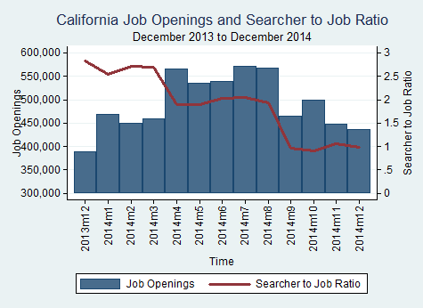
The number of job openings in California decreased from 436,019 in December 2014 to 425,877 in January 2015. The median number of job searchers per job opening across all MSAs (metropolitan statistical areas) and occupations in California was 0.98 in December 2014 and 1.77 in January 2015.
Month: April 2015

Texas job openings by major occupational group for January
Texas January 2015
Total number of job openings and median searcher-to-job ratio across all MSAs (metropolitan statistical areas) for each major occupational group in Texas in January 2015.
| Occupation | Job Openings | Searchers-to-Job Ratio |
| Management, business, and financial occupations | 56,662 | 0.58 |
| Professional and related occupations | 83,549 | 0.67 |
| Office and administrative support occupations | 55,482 | 0.89 |
| Sales and related occupations | 30,126 | 1.18 |
| Service occupations | 64,965 | 1.42 |
| Installation, maintenance, and repair occupations | 18,437 | 1.48 |
| Transportation and material moving occupations | 19,703 | 1.67 |
| Production occupations | 21,721 | 2.09 |
| Farming, fishing, and forestry occupations | 937 | 5.4 |
| Construction and extraction occupations | 14,583 | 5.44 |
Source: BLS
A narrative description of the Millimet et. al (2002) econometric worklife model
The following describes the approach used by Millimet et al (2002) to estimate U.S. worker worklife expectancy. The pdf version can be found here: Millimet (2002) Methodology Description
Methodology
First, transition probabilities are obtained from a two state labor market econometric model. The two labor market states are active and inactive in the workforce. The transition probabilities are the probabilities of going from one labor market state to another, such as active in one period and inactive in the next period. There are four such transition probabilities (Active-Active, Active-Inactive, Inactive-Active, Inactive-Inactive). The transition probabilities are obtained from the conditional probabilities estimated using a standard logit frame work. The logit model states:

Where y is equal to 1 if the individual is active and y equals 0 if the individual is inactive in the workforce during the period. Logit regression models are estimated separately for active and inactive individuals. For example, for a person who is initially active, the two estimated transition probabilities (Active to Active and Active to Inactive) equations are:

The estimated transition probabilities for persons who are initially inactive are estimated in a similar manner. The transition probabilities/conditional probabilities are used to construct predicted transition probabilities for each individual in the data set.
The average of the individual predicted probabilities for each age are ultimately used to calculate the transition probabilities in the Millimet et al. (2002) econometric worklife model. The average predicted transition probabilities at each age are:

In the calculation the averages are weighted by the CPS weights. Also anine year moving average is used to smooth out the transition probabilities.
The worklife expectancy at each age can be determined recursively. Specifically, if there is an assumed terminal year (T+1) in which no one is in the workforce, then the worklife expectancy for each age prior can be determined by working backwards in the probability tree. For instance at the terminal year, the individual’s worklife in the terminal year is the worklife probability in that terminal year. For example, assume that after age 80 no individuals are active in the work force. In this example, the probability that a person who is active at age 79 will be active at age 80, is the worklife expectancy for the individual at age 79. As described below this fact allows the worklife for all ages to be determined recursively using the transition probabilities obtained from the logistic regression models.
So specifically, the worklife () is the probability that the person active at time T remains active at the beginning of period T+1 (or end of T). It is assumed that no one is active after time period T+1. Similarly, the worklife () is the probability that the person inactive at time T is active at the beginning of period T+1 (or the end of T). Accordingly, there are multiples ways that a person at the end of time period T-1 can arrive at being active or inactive at the end of T, the terminal year. For instance, the person could be active in T-1 and then active in T. The transition probability for the is person is: . Alternately the person could be inactive in T-1 and active in T. The transition probability for this person is Two similar transition probabilities can be obtained for persons who are initially inactive at time T-1.
Using the worklife expectancies( and ) for the year prior to the terminal year can be calculated using the four transition probabilities described above. Specifically the worklife expectancies are as follows.
l
The 0.5 factor is included to account for the assumption that all transitions are assumed to occur at mid year.
Using this methodology, the worklife expectancy for each year prior to the terminal year in a recursively fashion.
All four largest MSAs in Texas see annual increase in job openings for Jan


Compared to December of last year, all of the main MSAs (metropolitan statistical areas) in Texas saw an annual increase in the number of job openings and in the searcher-to-job opening ratio.
Source: BLS
All four largest MSAs in Texas see annual increase in job openings for Jan
Compared to December of last year, all of the main MSAs (metropolitan statistical areas) in Texas saw an annual increase in the number of job openings and in the searcher-to-job opening ratio.
Source: BLS
Texas job openings increased from Dec to Jan
The number of job openings in Texas decreased from 270,849 in December 2014 to 366,165 in January 2015. The median number of job searchers per job opening across all MSAs (metropolitan statistical areas) and occupations in Texas was 0.56 in December 2014 and 1.09 in January 2015.

Source: BLS