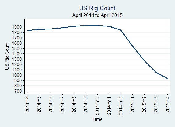
The U.S. rig count was 932 in April 2015, down from 1,048 in March 2015; Texas rig count was 393 in April 2015, down from 462 in March 2015; The Eagle Ford Shale rig count was 115 in April 2015, down from 137 in March 2015.

Source:Baker Hughes
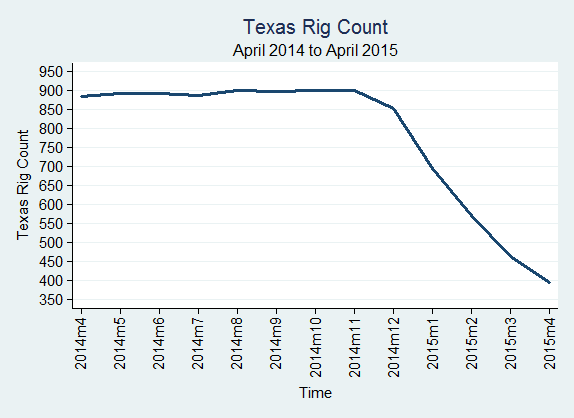
The U.S. rig count was 932 in April 2015, down from 1,048 in March 2015; Texas rig count was 393 in April 2015, down from 462 in March 2015; The Eagle Ford Shale rig count was 115 in April 2015, down from 137 in March 2015.
Source:Baker Hughes
That’s a question that comes up a lot in wage and hour land employment lawsuits. Typically the question is how many employees do I need to look at to have a statistically significant sample?
 In some instances it’s not feasible to collect data or get all the records for
all the employees of a particular company. Sometimes the data is kept
in such a way that it takes a lot of effort to get that information. In
other instances it is a matter of the limitations of imposed by the court.
In any event, that’s a question that comes up a number times in wage and hour lawsuits particularly ones involving class or collective actions. So what’s the answer?
Generally, the size of the sample needs to be sufficiently large so that it is representative of
the entire employee population. That number could be relatively small say 40 employees or relatively large say to 200 employees depending on the number of employees at the company and the characteristics of the employee universe that is being analyzed.
For example if there are no meaningful distinctions between the employees in the universe, that is
it is generally accepted that all the employees are pretty much all
similarly situated, then a sheer simple random sample could be
appropriate.
That is, you could simply draw names from a hat, essentially. A simple random sample typically requires the smallest number of employees.
If there are distinctions between employees that need to be accounted for, then
either a larger sample or some type of stratified sampling could be appropriate.
Even if there are distinctions between employees, if the sample is sufficiently large then distinctions between the employees in the data could take care of themselves.
For instance, assume that you have a population of 10,000 employees and they are
divided into four different groups that need to be looked at differently.
One way to do a sample in this setting is to sample over each of the different groups of employees separately. The main purpose of the individual samples is to make sure that you have the appropriate number of employees in each of the different groups. That is, to make sure that the number of employees in the different samples are sufficiently representative of the distribution of the different groups of employees in the overall population.
Another way to do this is to simply just take a large enough sample so that the distinctions take care of themselves. If the sample is sufficiently large then the distribution of the different groups of employees in the sample should on be representative of the employee population as a whole.
So in this example, if there is a sufficiently large sample it could be okay to use a simple random sample and you would get to the same point as a more advanced stratified type of approach.
The key however is to make sure that the sample is sufficiently large that of course depends on the overall population and the number of groups of employees being studied.
Update of our Mexican work life paper on the way!
We’re pleased to let you know that we have released our most current database: MMP150. The MMP150 database consists of 150 communities, which includes the original 143 communities plus 7 new additional communities: 4 from the state of Jalisco and 3 from the state of Puebla. MMP150 – PERS file provides individual level data for 157,879 persons; the MMP150 – MIG file provides detailed information about 8,052 heads of households with migration experience to the U.S; and the MMP150 – HOUSE file provides information about 24,989 households. The COMMUN file now provides homicide rates at the municipio level from 1990 to 2013.
MMP150 databases are available in SAS, Stata, SPSS, and also on CSV. To access these datasets, please visit the OPR’s archive webpage. We will be updating both the NATLYEAR and NATLHIST files over the summer.
http://mmp.opr.princeton.edu/databases/dataoverview-en.aspx

Median rent rose in San Antonio, Laredo, and Corpus Christi from January 2015 to February 2015.

Median house prices for all three MSAs (metropolitan statistical areas) rose from January 2015 to February 2015.

Image source: http://www.asemooni.com/news/economic-news/the-president-agreed-with-the-increase-in-housing

 The consumer price index (CPI) went up from 234.677 in January 2015 to 235.186 in February 2015, an annualized rate of 2.60%.
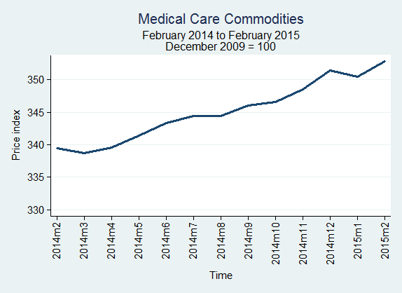
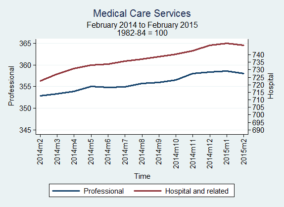
The price index for medical care commodities went down at an annualized rate of 0.06% from January 2015 to February 2015. During the same period, the price index decreased for medical care services (2.31%), hospital and related services (2.32%), and professional services (1.86%).
Source: BLS
Image source: http://www.shutterstock.com/pic-54762670/stock-photo-background-concept-illustration-consumer-price-index.html

WTI crude oil price decreased from $49.84 per barrel in February 2015 to $48.66 per barrel in March 2015. Natural gas price fell from $2.79 per million BTU (one million BTU is approximately 974 cubic feet) in February 2015 to $2.64 per million BTU in March 2015.

Texas crude oil production for January 2015 was 68,949,268 barrels, down from 77,599,222 barrels reported in December 2014. Texas natural gas production was 607,631,634 Mcf (thousand cubic feet) of gas in January 2015, down from the December 2014 gas production total of 674,495,129 Mcf.
Sources: eia.gov, rrc.state.tx.us

The number of job openings in Texas for nurses, therapists, and physician assistants increased from 10,144 to 10,588 from December 2014 to January 2015. The searcher-to-job opening ratio increased from 0.63 to 0.91 during that same span.

Source: BLS
Image source: http://www.carrollhs.org/s/1253/index.aspx?pgid=877

The health care and social assistance industry gained 3,000 jobs from January 2015 to February 2015. Compared to February 2014, the cumulative number of jobs added in this industry is 43,500, an annual increase of 3.3%.
Source:http://www.tracer2.com/admin/uploadedPublications/2133_TLMR-March_15.pdf
Image source: http://blogs.wsj.com/health/2012/01/06/health-care-sector-adds-jobs-as-overall-employment-picture-looks-healthier/
The STATA code for estimating the Millimet et a;. (2002) econometric worklife model can be found below. The code will need to be adjusted to fit your purposes. However, the basic portions are here.
use 1992-2013, clear
drop if A_W==0
keep if A_A>=16 & A_A<86
*drop if A_MJO==0
*drop if A_MJO==14 | A_MJO==15
gen curr_wkstate = A_W>1
lab var curr_wkstate “1= active in current period”
gen prev_wkstate = prev_W>1
lab var prev_wkstate “1= active in previous period”
gen age = A_A
gen age2 = age*age
gen married = A_MA<4
gen white = A_R==1
gen male = A_SE==1
gen mang_occ = A_MJO<3
gen tech_occ = A_MJO>2 & A_MJO<7
gen serv_occ = A_MJO>6 & A_MJO<9
gen oper_occ = A_MJO>8
gen occlevel = 0
replace occlevel = 1 if mang_occ==1
replace occlevel = 2 if tech_occ==1
replace occlevel = 3 if serv_occ==1
replace occlevel = 4 if oper_occ ==1
gen lessHS = A_HGA<=38
gen HS = A_HGA==39
gen Coll = A_HGA>42
gen someColl = A_HGA>39 & A_HGA<43
gen white_age = white*age
gen white_age2 = white*age2
gen married_age = married*age
gen child_age = HH5T*age
/*
gen mang_occ_age = mang_occ*age
gen tech_occ_age = tech_occ*age
gen serv_occ_age = serv_occ*age
gen oper_occ_age = oper_occ*age
*/
merge m:1 age using mortalityrates
keep if _m==3
drop _m
gen edlevel = 1*lessHS + 2*HS + 3*someColl + 4*Coll
save anbasemodel, replace
*/ Active to Active and Active to Inactive probabilities
local g = 0
local e = 1
forvalues g = 0/1 {
forvalues e = 1/4 {
use anbasemodel, clear
xi: logit curr_wkstate age age2 white white_age white_age2 married married_age HH5T i.year_out if prev_wk==1 & male==`g’ & HS==1
*Gives you conditional probability
*summing these figures gives the average predicted probabilities
predict AAprob
keep if occlevel==`e’
*collapse (mean) AAprob mortality, by(age)
collapse (mean) AAprob mortality (rawsum) MARS [aweight=MARS], by(age)
gen AIprob = 1-AAprob
replace AAprob = AAprob*(1-mortality)
replace AIprob = AIprob*(1-mortality)
save Active_probs, replace
*Calculates Inactive first period probabiliteis
use anbasemodel, clear
xi: logit curr_wkstate age age2 white white_age white_age2 married married_age HH5T i.year_out if prev_wk==0 & male==`g’ & HS==1
predict IAprob
keep if occlevel==`e’
*collapse (mean) IAprob mortality , by(age)
collapse (mean) IAprob mortality (rawsum) MARS [aweight=MARS], by(age)
gen IIprob = 1-IAprob
save Inactive_probs, replace
*Calculates WLE for Active and Inactive
merge 1:1 age using Active_probs
drop _m
order AAprob AIprob IAprob IIprob
*Set the probablilties for end period T+1
*Note the top age changes to 80 in the later data sets
gen WLE_Active = 0
replace WLE_Active = AAprob[_n-1]*(1+AAprob) + AIprob[_n-1]*(0.5 + IAprob)
gen WLE_Inactive = 0
replace WLE_Inactive = IAprob[_n-1]*(0.5+AAprob) + IIprob[_n-1]*IAprob
gen WLE_Active_2 = 0
replace WLE_Active_2 = WLE_Active if age==85
gen WLE_Inactive_2 = 0
replace WLE_Inactive_2 = WLE_Inactive if age==85
local x = 1
local y = 80 – `x’
forvalues x = 1/63 {
replace WLE_Active_2 = AAprob*(1+WLE_Active_2[_n+1]) + AIprob*(0.5 + WLE_Inactive_2[_n+1]) if age==`y’
replace WLE_Inactive_2 = IAprob*(0.5 + WLE_Active_2[_n+1]) + IIprob*WLE_Inactive_2[_n+1] if age==`y’
local x = `x’ + 1
local y = 80 – `x’
}
keep age WLE_Active_2 WLE_Inactive_2
rename WLE_Active_2 WLE_Active_`g’_`e’
rename WLE_Inactive_2 WLE_Inactive_`g’_`e’
save WLE_`g’_`e’, replace
keep age WLE_Active_`g’_`e’
save WLE_Active_`g’_`e’, replace
use WLE_`g’_`e’, clear
keep age WLE_Inactive_`g’_`e’
save WLE_Inactive_`g’_`e’, replace
di `e’
/**End of Active to Active and Active to Inactive probabilities*/
local e = `e’ + 1
}
local g = `g’ + 1
}
local g = 0
local e = 1
forvalues g = 0/1 {
forvalues e = 1/4{
if `e’ == 1 {
use WLE_Active_`g’_`e’, clear
save WLE_Active_`g’_AllOccLevels, replace
use WLE_Inactive_`g’_`e’, clear
save WLE_Inactive_`g’_AllOccLevels, replace
}
if `e’ > 1 {
use WLE_Active_`g’_AllOccLevels, replace
merge 1:1 age using WLE_Active_`g’_`e’
drop _m
save WLE_Active_`g’_AllOccLevels, replace
use WLE_Inactive_`g’_AllOccLevels, replace
merge 1:1 age using WLE_Inactive_`g’_`e’
drop _m
save WLE_Inactive_`g’_AllOccLevels, replace
}
local e = `e’ + 1
}
if `g’ ==1 {
use WLE_Active_0_AllOccLevels, clear
merge 1:1 age using WLE_Active_1_AllOccLevels
drop _m
save WLE_Active_BothGenders_AllOccLevels, replace
use WLE_Inactive_0_AllOccLevels, clear
merge 1:1 age using WLE_Inactive_1_AllOccLevels
drop _m
save WLE_Inactive_BothGenders_AllOccLevels, replace
}
local g = `g’ + 1
}
!del anbasemodel.dta

The oil and gas extraction industry in Texas lost 1,100 jobs from January 2015 to February 2015. Compared to February 2014, the cumulative number of jobs added in this industry is 1,400, an increase of 1.4%.
Source: http://www.tracer2.com/admin/uploadedPublications/2133_TLMR-March_15.pdf
Image Source: http://www.eliteexploration.com/texas-oil-gas-companies/