Accounting for kids and marriage in the calculation of a person’s worklife expectancy

Abstract (From Millimet et. al)

Measuring an individual’s human capital at a point in time as the present actuarial value of expected net lifetime earnings has a lengthy history. Calculating such measures requires accurate estimates of worklife expectancy. Here, worklife estimates for men and women in the USA categorized by educational attainment, race, marital status, parental status and current labour force status are presented. Race has a much larger impact on the worklife expectancy of men than women. Education is associated with larger worklife differentials for women. The association between marriage and worklife expectancy is significant, but of opposite sign, for men and women: married women (men) have a lower (higher) worklife expectancy than single women (men). Parenthood is associated with a reduction in the worklife expectancy of women; the association is smaller and varies from positive for some education/marital status groups to negative for others for men.

From:

DETAILED ESTIMATION OF WORKLIFE EXPECTANCY FOR THE MEASUREMENT OF HUMAN CAPITAL: ACCOUNTING FOR MARRIAGE AND CHILDREN
Daniel L. Millimet
Southern Methodist University
Michael Nieswiadomy
University of North Texas
Daniel Slottje
Southern Methodist University:


Steps to converting non-analyzable wage, time, and business electronic data

When manual data entry of non-analyzable financial or wage data  is not an option, OCR software and specialized designed and written computer software data cleaning routines is a good alternative.
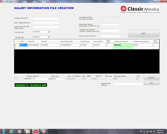
For example in our approach, we use a number of OCR programs including Abbey Reader to first translate the data into a format that is recognized by statistical programs such as STATA and computer software script languages such as VBA.

Once the data is converted, we write specialized computer software routines to extract the relevant data from the converted file.  The computer code, which is written in STATA, VBA, or other scripting language, puts the extracted data into a format that can be analyzed by statistical and spreadsheet programs.

These approach to converting wage, business, employment or other types of data has the advantage of being able tobe  reproduced by either party if required.

Having both the data cleaning and statistical and economic analysis performed by the same economic outfit and team is desirable.  Data cleaning is not performed in a vacuum; that is the very definition of ‘dirty data; depends on what the data is to be used for.  Some data items may not convert very well by the OCR and software code, but the items may be of little value in the economic and statistical analysis in the first place.

One advantage of using the same research outfit to do both the data cleaning and the economic and statistical analysis is that the distinction gets made early in the analysis process.


Converting and analyzing wage and business data from PDFs

Some wage and business data is electronic but is not analyzable in the format that it is maintained by the employer or company.

For instance,some employers use computerized data systems for recording the start times, lunch periods, and end periods for certain employees.  When reviewing this data in the regular course of business some of these employers review standardized, pre-formatted reports of the time punch data instead of the actual underlying time punches that were made by each individual employee.  Many of these standardized reports are presented in a PDF or other non-analyzable electronic format.

Similarly, some businesses retain certain information, such as itemized copies of purchase orders, only in a PDF or other non-analyzable electronic format.

The task when addressing economic damage issues that rely on this type of non-analyzable electronic information, is to accurately and efficiently translate the data into a format that can analyzed using statistical programs, such as STATA.  In cases with relatively small amounts of data spreadsheet programs such as EXCEL could also be used.

How is this done? Next>>>>

Employer Labor Hoarding Part I:What is it?

20140502-130044.jpg

Labor hoarding is a concept where employers hold onto workers during economic down times even though they don’t necessarily need them. The idea is that the cost of retraining employees is sufficiently high that it is more cost-effective for employers to retain employees even though they are under utilized.

Initially the concept of labor hoarding was used to explain an apparent contradiction in the economic literature.

The economic contradiction was that during economic expansions employers would not necessarily hire more people. Also it was observed that employers were not necessarily releasing employees when downturns occurred.

This observation also led to a apparent contradiction in the labor economic literature.

According to labor economic literature the average productivity of labor should increase during slowdowns and recessions. The fall of average productivity theoretically, would occur because firms would reduce their labor force during recessions and employees essentially would do more with less during economic contractions.

So for example, delivery workers would be assigned to additional routes during a contraction and instead of having two people cover two routes, the routes would be consolidated so that only one person would be needed.

Since the production level is the same (or least falling at a slower rate than the decline in workers) and the number of workers declines, the average productivity of labor would increase. Alternatively the marginal productivity of labor would increase since fewer workers are needed. (Recall, that there is a inverse relationship between the marginal productivity of labor and the number of workers.)

So what does the current economic literature say about labor hoarding?

Three takeaways from a closer look at job openings data for March 2014

The Conference Board Help Wanted Online (HWOL) data series release for March 2014 indicated a number trends worth discussing.

The Conference Board Help Wanted OnLine® Data Series (HWOL) measures the number of new, first-time online jobs and jobs reposted from the previous month for over 16,000 Internet job boards, corporate boards and smaller job sites that serve niche markets and smaller geographic areas.

The Conference Board’s HWOL series measures help wanted advertising, i.e. labor demand. The HWOL data series began in May 2005. The HWOL provides seasonally adjusted data for the U.S., the nine Census regions and the 50 States. The HWOL also provides seasonally adjusted data for occupations and for the 52 largest metropolitan areas..

So what are the trends.  Three take aways

  • Shale drilling influences remain high.   The state of North Dakota, which has a very active Shale play,  had one of the lowest supply to demand ratios (S/D ratio) of 0.46.  That is there were over 2 jobs advertised for each available worker.  Texas and the metro areas in Texas also had high employer demand.
  • California economy is growing again but in spurts. Some metro areas in California such as San Jose had a very high employer demand (1.31 S/D ratio) while others like Riverside had a lot of searchers per job opeing (5.15)
  • STEM rules.  Computer, math, and engineering jobs are in high demand.  The HWOL data shows that many of these occupations have S/D ratios of less than one

Affordable Care Act changes high risk health insurance coverage in Texas

Like many states, up until the passage of the Affordable Care Act, Texas maintained a separate insurance pool for high risk individuals who could not obtain insurance from another source.

In Texas, that pool was known as the Texas Health Insurance Pool.  The Texas Health Insurance Pool insured individuals, such as those with pre-existing conditions, who could not obtain insurance from other sources.   As would be expected, the premiums, which reflect the higher health risk of the insured, offered by the Texas Health Insurance Pool were significantly higher than the rates offered by non-high risk insurance companies.

The Affordable Care Act and the Health Exchanges have changed high risk health insurance in Texas.  The Texas Health Insurance Pool no longer offers insurance policies and refers those individuals to health.gov for enrollment in the Federal Insurance Market system.

So how do the rates compare?  The rates under the Affordable Care Act are generally lower than the rates offered by the old Texas Health Insurance Pool.  For instance, consider a 53 year old, male smoker who had pre-existing health issues.  If this person were to select a gold level plan under the Affordable Health Care Act, which does not take the pre-existing conditions into account, they could expect to pay about $850 a month.  The same person would have paid about $1,500 a month under the old Texas Health Insurance Pool.

U.S. BLS data provides a closer look at what 27 year olds are doing today at work, school, and home

The U.S. BLS released some interesting statistics on what people born in the early 1980’s are doing today in the labor market, school, and at home. The findings are from the National Longitudinal Survey of Youth 1997, a nationally representative survey of about 9,000 young men and women who were born during the years 1980 to 1984

Here are some of the major findings.

Women have more education: By 27 years of age, 32 percent of women had received a bachelor’s degree, compared with 24 percent of men. Nine percent of men were high school dropouts compared to 8 percent of women.

Everybody changes jobs a lot!.  Individuals born from 1980 to 1984 held an average of 6.2 jobs from ages 18 to 26. The
number of jobs held varies by education for women but not for men.

•Those without HS have a hard time getting a job.   High school graduates who had never enrolled in college were employed an average of 68 percent of the weeks from ages 18 to 22, and 74 percent of weeks from ages 23 to 26. In comparison, those who had dropped out of high school were employed 51 percent of weeks from ages 18 to 22, and 57 percent of weeks from ages 23 to 26.

Most are not married. Thirty-four percent of young adults were married at age 27, while 20 percent were cohabiting and 47 percent were single. On average, young adults with more education were more likely to be married and less likely to be cohabiting. Young adults who were single at age 27 were employed 70 percent of the weeks from ages 18 to26, compared to 77 percent of weeks for those who were married and 72 percent of weeks, for those who were cohabiting.

• The moms work outside of the home. Women with children in their household at age 27 were employed 65 percent of weeks from age 18 to 26 compared to 76 percent of weeks for women without children in their home. Conversely, men tended to work more weeks if they had children in the household than if they did not (79 percent of weeks versus 73 percent).

Work life cycle labor market model shows lifetime impact of Great Recession on earnings and wages

assemblers2


The graph above shows the expected lifetime earnings of a person working as a manufacturing assembler.  The red line shows the earnings that a person who began working as a manufacturing assembler in 2006 could expect over their projected work life of approximately 44 years.   The blue line shows the earnings that a person who began working as a manufacturing assembler in 2010 could expect over a projected work life of approximately 44 years.  Both projected earnings streams account for projected inflation.

The work life earnings for manufacturing assemblers, projected using a life cycle labor market model, show that after the Great Recession these types of workers can expect both lower annual earnings and wage increases over their projected working life.

Methodology:

The projected earnings profiles are constructed from statistical models based on the Current Population Survey (CPS) labor market data from the U.S. Bureau of Labor Statistics (BLS).  The earnings profiles for assembly workers are based on the earnings of high school educated white male assemblers and fabricators, working full-time or part-time, in 2006 and 2010.

Total U.S. employment levels nearly at pre-recession level; expected to reach by mid summer.

U.S. employment almost at pre-recession levels

Total U.S. employment is nearly at it’s pre-recession level.  Right at the beginning of the recession total non-farm U.S. employment, which includes about 80% of all workers, was a little over 138,000,000.  Right now total non-farm U.S. employment is a little under 138,000,000.

Generally, non-farm employment is subject to fluctuations such as seasonal changes in weather, major holidays, and the opening and closing of schools.   However, at the current rate of growth, U.S. employment can be expected to reach pre-recession levels by mid summer.

For more see:

(1) Bureau of Labor Statistics. “Employment, Hours, and Earnings from the Establishment Survey.” BLS Handbook of Methods; last date modified July 10, 2013; http://www.bls.gov/opub/hom/.

Atlanta Fed President suggest that U.S. labor market has a ways to go before reach full employment; especially the shadow work force

Atlanta Fed President
In a recent speech, the Atlanta Fed Pres. suggested that the U.S. labor market has a ways to go before reaching full employment. He was especially concerned about re-engaging the workers in the ‘shadow labor market’.

The shadow labor market includes people who are still willing to work but have essentially stopped looking for work. The BLS provides some measure of this in its U-6 measure of unemployment.

As this graph shows, U6, which accounts for the shadow workers, runs at about 2x the rate of the official unemployment rate. The Atlanta Fed Pres. statements show particular concern for reabsorbing (or simply put, getting jobs for) these individuals into the workforce.